
Home |
Tutorial |
Theory |
References |
ENM 1.0 |
ANM 2.0 |
Computational & Systems Biology |
NTHU site
|
|
|
Home |
Tutorial |
Theory |
References |
ENM 1.0 |
ANM 2.0 |
Computational & Systems Biology |
NTHU site
|
Tutorial for Gaussian Network Model Database (GNM-DB) – iGNM 2.0
2.3. Domain Separations by Dynamics
2.6. Collectivity of slow modes
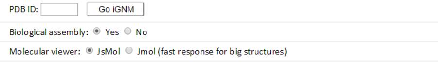
Enter the PDB ID (e.g., 101M) and click the “Go iGNM” button to submit a query to GNM database.
Both the GNM results for the biological assembly (BA) and the structure in the asymmetric unit (the default structure) are provided in the current GNM database. The GNM results for BAs are the default querying targets. Jsmol is the default molecular visualizer for viewing the PDB structures color-coded by the size of motions in individual GNM modes or all modes. To view the structures with Jmol, instead, the up-to-date Java Runtime Environment is required. Please click the “Run” and “Allow” buttons to run Jmol when the security warning displayed below pops up:
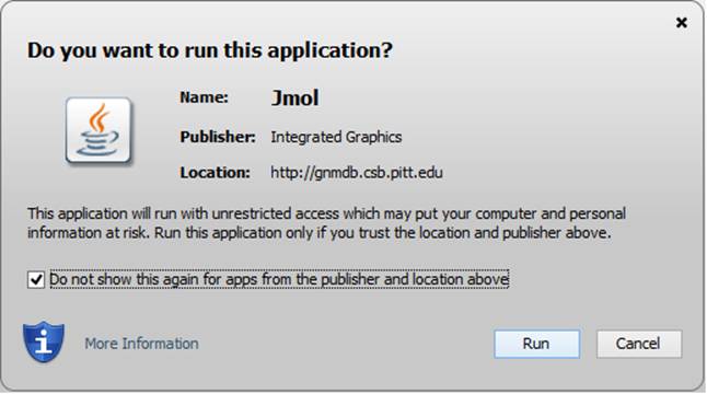
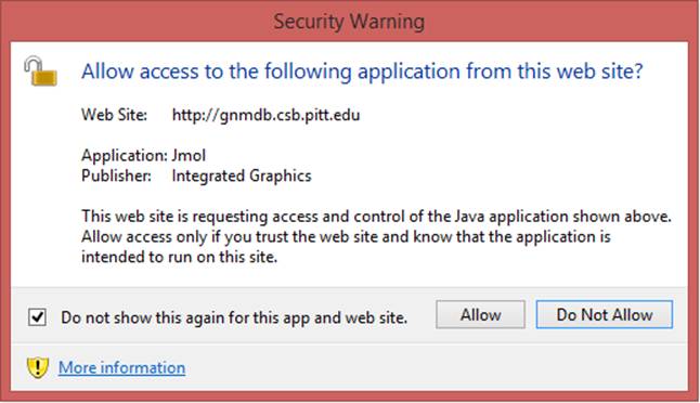
We recommend to check the box “Do not show this again for this app and website” before clicking the “Run” and “Allow” buttons, to avoid seeing this window in future applications.
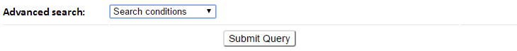
Select the search conditions (e.g., Experiment Method, dynamics properties) from the advanced search drop-down button.
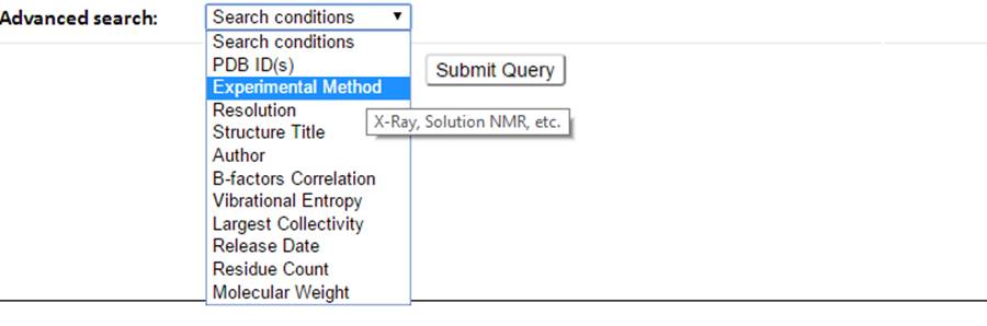
The corresponding input forms for each selectable item will show.
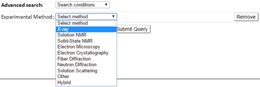
11 queryable items including the PDB features such as PDB ID, Experimental Method, Resolution, Structure Title, Author, Release Date, Residue Count and Molecular Weight, and GNM-defined dynamics features such as B-factor correlation, Vibrational Entropy and Largest Collectivity can be selected and combined to define search conditions.
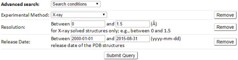
For example, a customized search conditions to search structures of a released date between 2000-01-01 and 2015-08-31 and a high resolution (≤ 1.5 Å) can be defined as the above combined conditions. The result page of which is shown below.
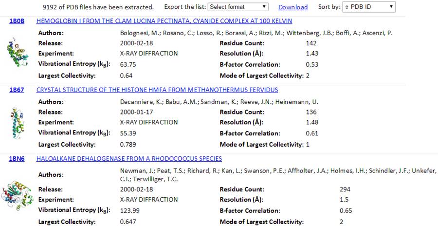
The total number of found PDB structures is listed in the top of the result pages. All the searched PDBs can be viewed online or downloaded. The searched results can be sorted by the PDB ID, Experimental Method, Residue Count or Resolution via clicking the “Sort by” drop-down options. The relational table can be downloaded using the “Export the list” drop-down button. Several formats (tsv, csv, xls and xlsx) can be selected.
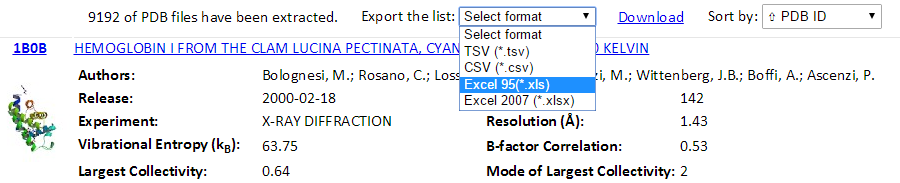
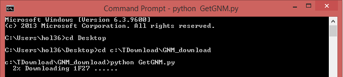
Also, a Python code “GetGNM.py” can be downloaded from the “Download” link. Executing the Python code GetGNM.py in command line would initiate the download of GNM results for the searched PDB hits. All the GNM results files will be downloaded in the current/work folder.
This page contains a J(s)mol window (left), Results panel and the input information (right).
The J(s)mol window displays the PDB structure colored based on the size of motions driven by the slowest two GNM modes (blue: almost rigid; and red: highly mobile, as indicated by the color code bar under the diagram).
Take the sperm whale myoglobin (PDB id: 101M) as an example. The corresponding Results page is displayed below.
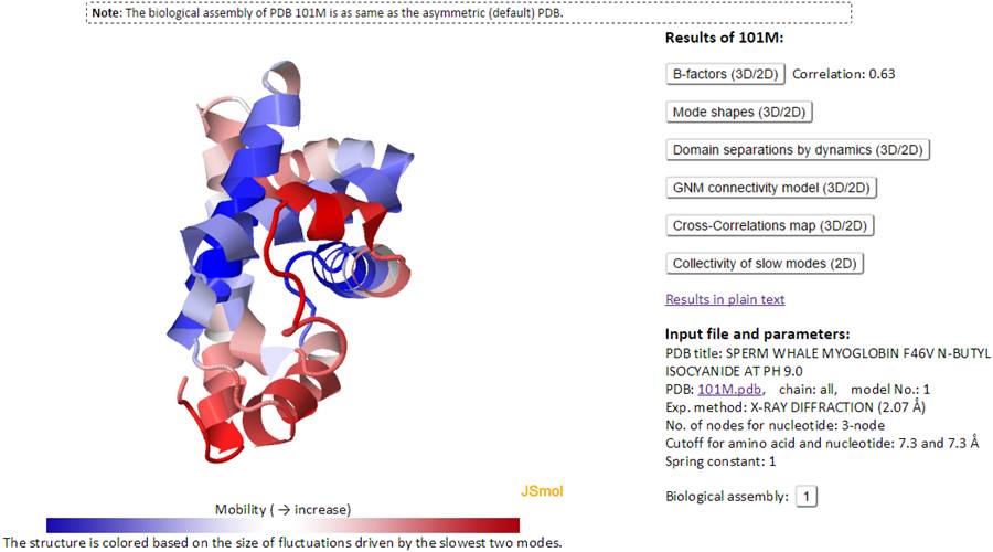
The Results panel contains seven clickable items:
1) B-factors (correlation between theoretical and experimental B-factors, for X-ray structures only)
2) Mode shapes
3) Domain separations by dynamics
4) GNM connectivity model
5) Cross-Correlations map
6) Collectivity of slow modes
7) Results in plain text
The input information (Input file and parameters) contains input PDB ID and parameters used for GNM calculations. For example, the computations for PDB 101M were performed for all chains in the Biological Assembly, using the first model deposited in the PDB (PDB: 101M.pdb, chain: all, model No.: 1); 101M structure was resolved by X-ray crystallography, at a resolution of 2.7 Å (Exp. method: X-RAY DIFFRACTION (2.07 Å)); three atoms P, C4' and C2 were selected as network nodes representing nucleotides (No. of nodes for nucleotide: 3-node). Note that the Cα atom was selected as the (single) node for each amino acid. Node pairs within cutoff distances of 7.3 and 7.3 Å are adopted for amino acid pairs and for nucleotide pairs, respectively (Cutoff for amino acid and nucleotide: 7.3 and 7.3 Å); the spring constant for contacting nodes is taken as unity, 1.
In addition, all the BA structures for a PDB entry are listed (see the example for PDB 3WZ5 that have 4 biological assemblies) under the input information panel. Only the first BA of the PDB was pre-calculated, if the PDB have more than 1 BA records.
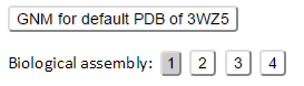
In the BA results page, the 2nd+ BA structures can be calculated via an online calculation engine by clicking the corresponding Biological assembly. The GNM results page can be viewed by clicking the button “GNM results for default PDB”.
For any PDB entry with the 1st BA that is identical to the structure in the asymmetric unit (the PDB default), the GNM results for the default structure will be used for the 1st BA.
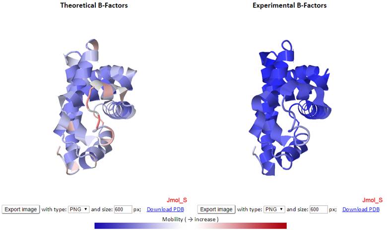
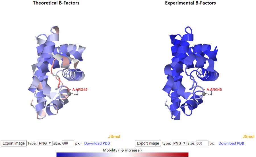
The theoretical and experimental B-factors are displayed/compared using both 3D color-coded PDB structures using J(s)mol and 2D interactive graphs. Corresponding PDB structure, color-coded by residue fluctuations (see below), can be downloaded from the “Download PDB” links.
In the 3D J(s)mol window, the structures are represented as cartoon and color-coded by GNM-defined theoretical fluctuations or X-ray solved experimental B-factors (the B-factor column in PDB files). The colors are defined by the mobility of the residues/nodes. Rigid and mobile residues are colored blue and red respectively.
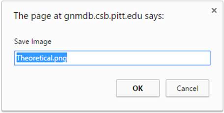
Click the “Export image” button to export images from the 3D J(s)mol windows with different image types (png, jpg and gif) and resolution (600 px for both width and height by default). The pop-up export dialog box for Jsmol is displayed as
while the export dialog box for Jmol has more functions:
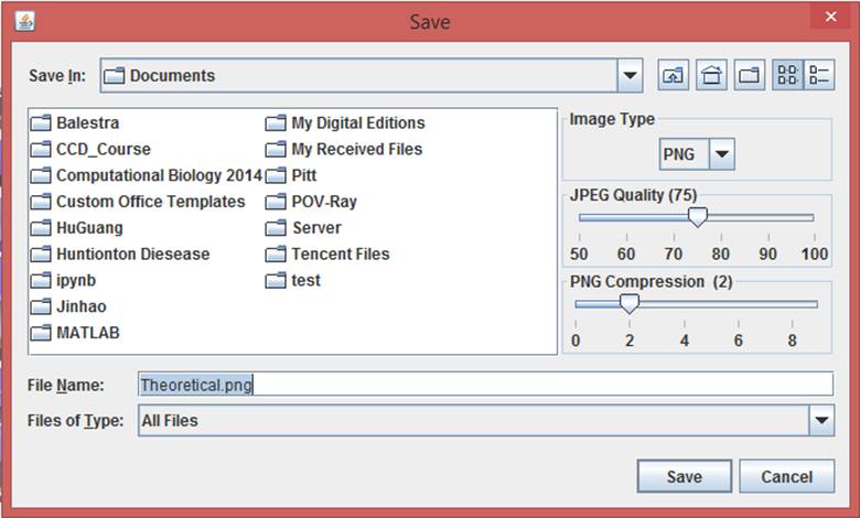
The image type, quality and compression can be selected with the dialog box.
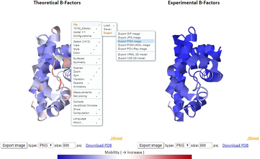
Right click the J(s)mol windows to show the menu, and more functions can be found in the pop-up J(s)mol menu:
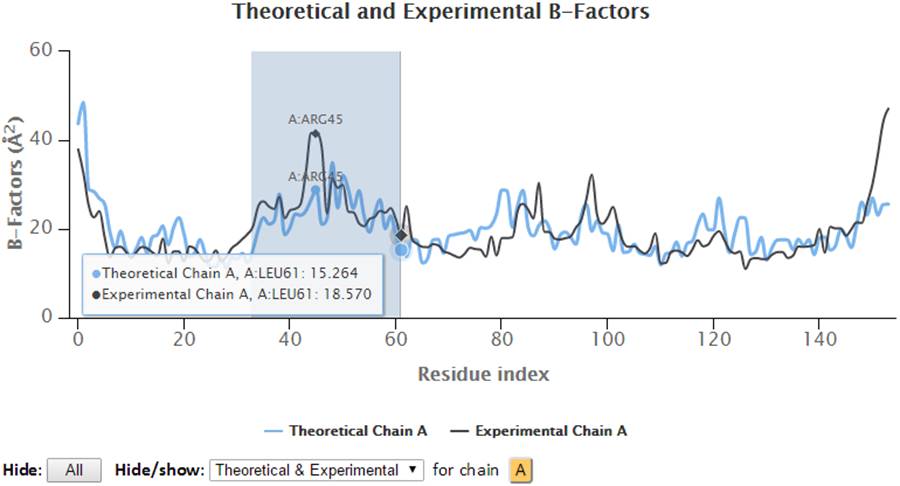
The 2D profiles of B-factors as a function of residue index are plotted using the interactive chart. The x- and y-axes refer to the residue index (ID) and B-factors respectively.
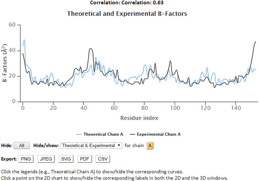
The control panel below the chart can be used to hide/show the specified chain(s) and charts (theoretical and/or experimental). Also, the legends can be clicked to hide or show the corresponding curves in the chart. Three formats of images (png, jpg and svg) and PDF document of the customized 2D charts can be exported using the “Export” buttons. Also, all the text data in csv format can be export using the “CSV” export button.
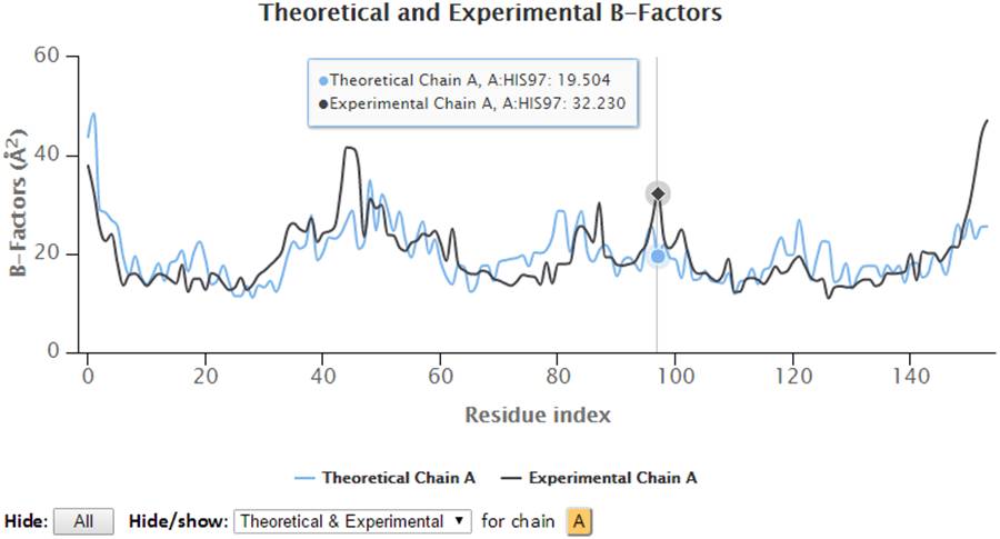
Hover on the plots will display the plotted series with their names, the residues information (chain identifier, residue type and residue ID) and corresponding B-factors.
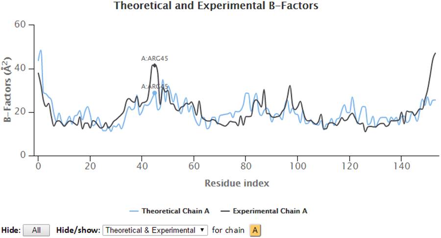
Besides, the points in the 2D graph can be clicked to label the corresponding residue in the 3D J(s)mol window where Cα atoms are presented in gray balls and sidechain atoms are in “wireframe”.
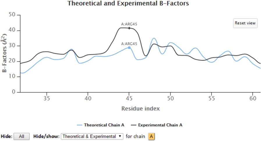
Select a range of the 2D chart will zoom in the chart to selected view and a “Reset view” button will pop up in order to restore the view to molecule’s full length upon clicking.
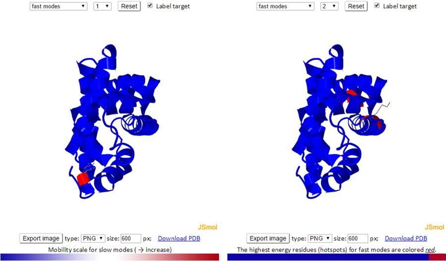
Similar to the B-factors results page, 3D J(s)mol windows and 2D interactive charts are provided to display the slow and fast modes along with the modes averages.
The 3D structure shown in J(s)mol is colored based on the mobility of the residues in a certain mode. The color spectrum goes from blue (most rigid) -> white -> red (most mobile).
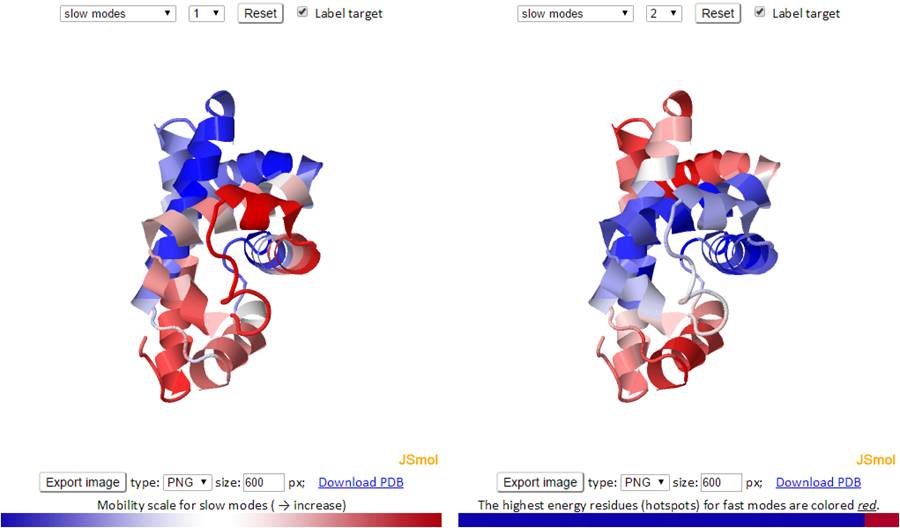
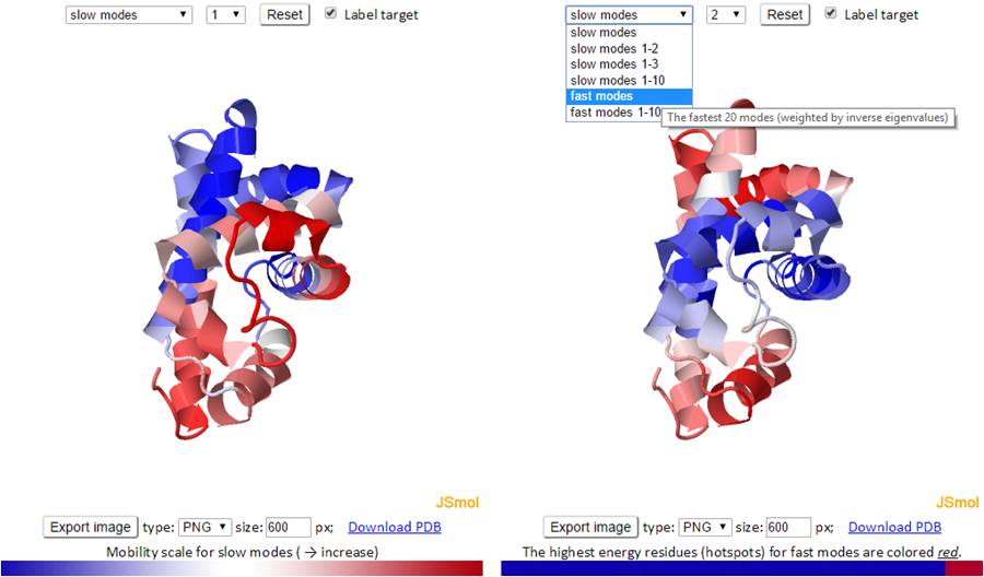
The mode types (individual slow modes, average of the slowest 1-2 or 1-3, fast modes and fast average 1-10) can be selected from the drop-down menu. The mode index can be selected only for the slow and fast modes. The default mode is the slow mode since the slow modes make the largest contribution to the fluctuation of the structure and usually correlate with biological function. The colors on the structure are updated automatically by changing the mode type or mode index. We provide two 3D windows for easy comparison between two modes.
For fast modes, the whole structure is colored blue except for the hot spot residues (those subjected to highest frequency fluctuations) which are colored red.
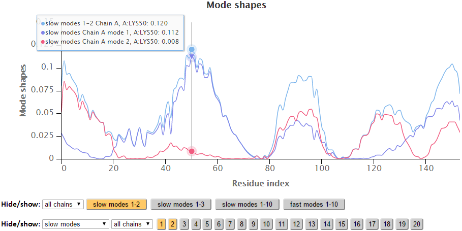
The modes in the 2D charts are scaled by the relative inverse of the eigenvalues of the Kirchhoff matrix (G). Similar to the B-factors results page, point labels and zoom in functionality are available for the interactive 2D chart. The Hide “All” button hides all the series in the chart making it easy to reset the chart.
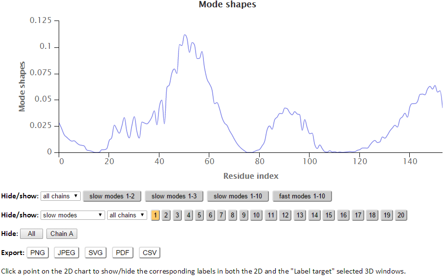
The export buttons provide different ways to export customized figures or data in different formats. The activated buttons has an orange colored background while inactive buttons has a gray background.
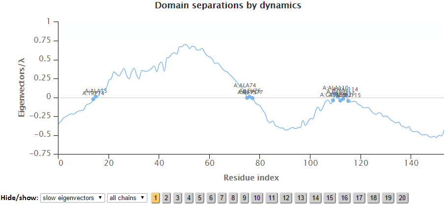
The residues are separated based on the sign (+/-) of each residue in an eigenvector. The residues with the same sign in the eigenvector moves together. The interfacial residues are shown using the wireframe representation. The 3D J(s)mol windows and the 2D interactive chart have the same functionality as the Mode Shapes result page.
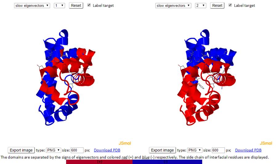
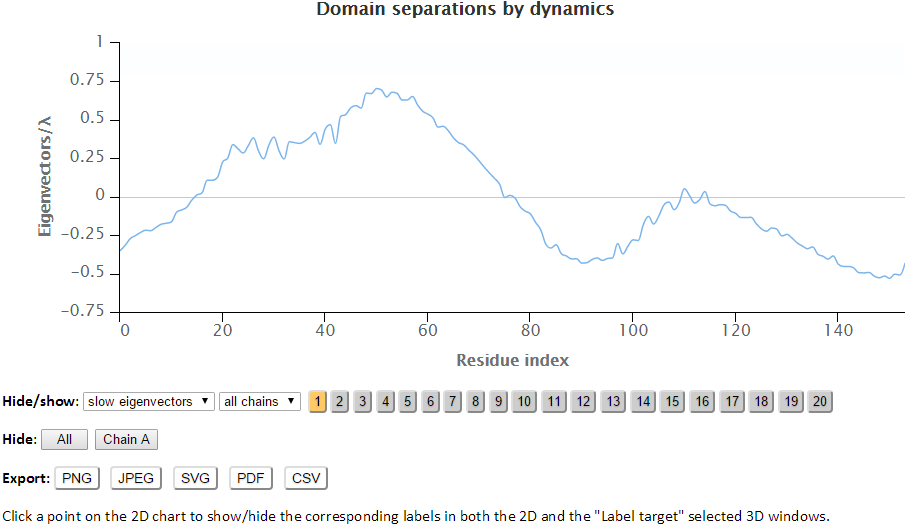
The labeled residues in the Domain Separation chart below are the interfacial residues whose neighboring residues have a different sign in the eigenvector relative to themselves. The interfacial residues act as hinges in the movement of the molecules.
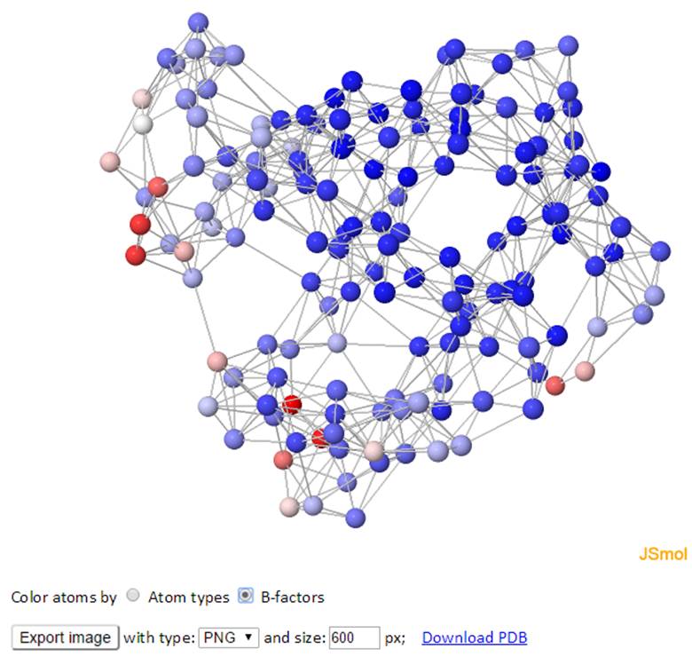
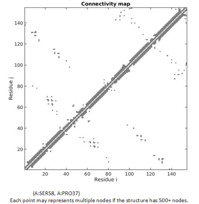
The network of the GNM model is displayed in both 3D structure and 2D connectivity map. Each ball represents a node and each line between the nodes represents a spring connection/interaction between the pair of interest if the pair stays within a cutoff distance in space.
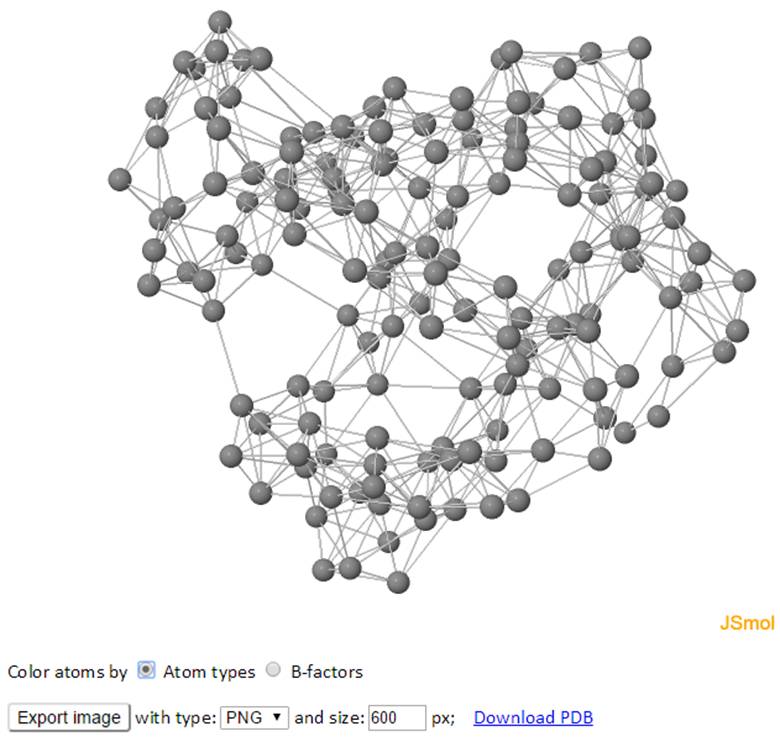
The color of atoms/nodes (balls) can be changed by clicking the radio button “Atom names” and “B-factors”. Similar to the 3D B-factors windows, images can be exported using the export button.
The topology of the network can also be viewed from the 2D Connectivity map. Each dot represents a spring connection between residue i and j. The residue information of the residue i and j can be displayed while hovering the cursor on points in the map.
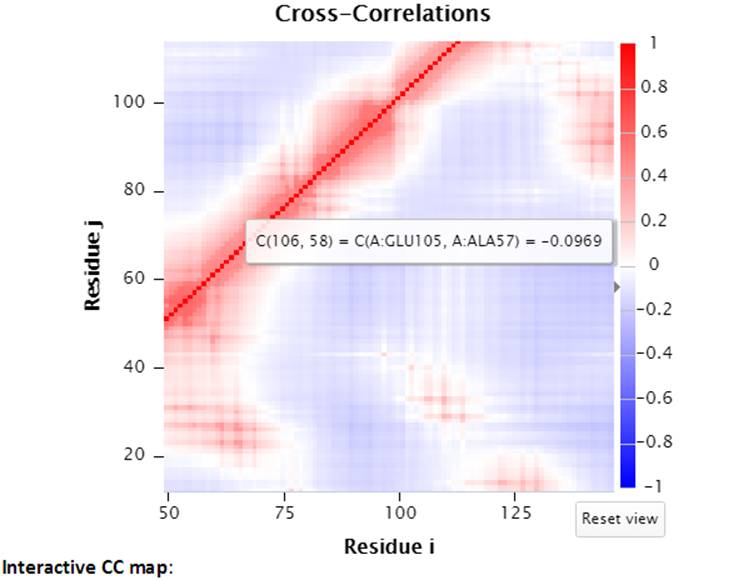
The Cross-Correlation (CC) map for all modes is provided by default. For PDB structures with less than 1000 nodes, the CC map can be customized with any range of modes. A customized CC map can be obtained by changing the range of modes and then clicking the “Calculate” button. Residue numbers (i,j) along the axes refer to those of all chains ordered by chain index.
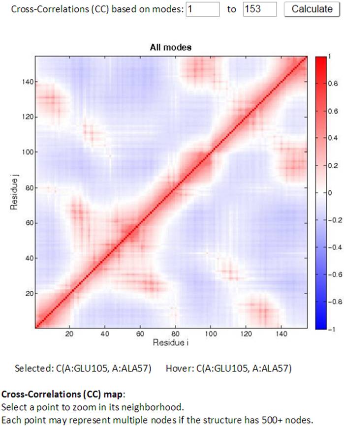
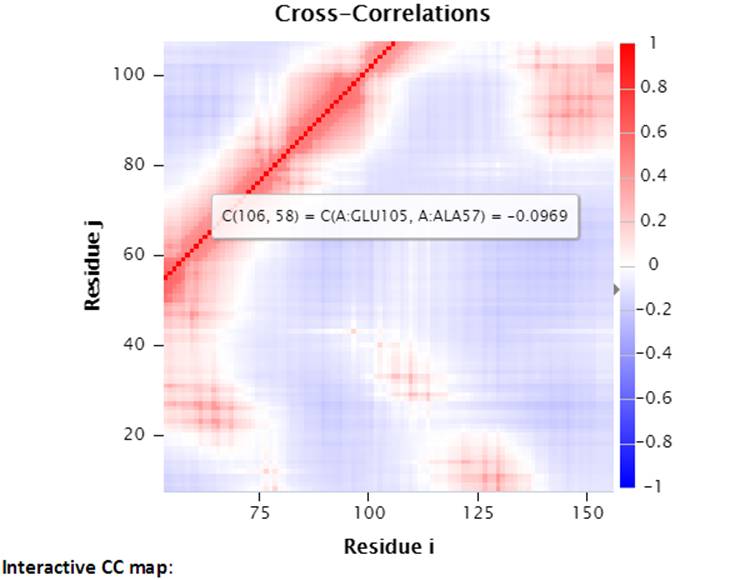
Two CC maps (static and interactive, on the left and right hand side respectively) are shown for those structures that have no more than 1,000 nodes. While the mouse hovers over the static (left) CC map, the information for the pair of residues of interest will be displayed below the map. By clicking a point in the static map, the interactive CC map will show the zoomed in view containing 100 residues on both axes centered at the selected point in the static map. The detailed information can be displayed well in the interactive CC map for the big structures.
An example of interactive CC map of PDB ID: 101M in action when a point (A:GLU105, A:ALA57) was selected in the static CC map:
The size of interactive CC map can be customized using the control panel below the map. The minimum residue indices i and j can be changed as well as the map size. The maximal indices are automatically calculated based on the minimal index and the map size (e.g., there are 100 points between min i 45 and max i 144). The “Redraw” button redraws the interactive CC map based on the settings (min i, j and the map size which define the map range) in the control panel. The following interactive CC map will be drawn using settings: map size = 100, min i = 45 and min j = 6.
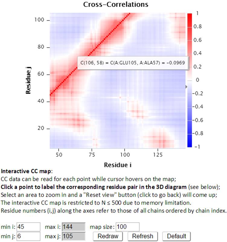
The “Refresh” button not only redraws the interactive CC map using the settings, but also reloads the page with a new URL address containing the new settings. For example, http://gnmdb.csb.pitt.edu/iGNM_CC_map.php?gnm_id=101M&modes=cc_all&x_min=45&x_max=144&axis_length=100&y_min=6&y_max=105&max_length=800 is the URL of the page generated by clicking the “Refersh” button using the above settings. The URL directly restores the customized view of the above interactive CC map therefore it can be saved/shared for later viewing. The “Default” button resets the settings to the default settings.
Furthermore, the interactive CC map can be zoomed in by selecting a range of points on the map. The “Reset view” button will reset the interactive CC map back to the original view.
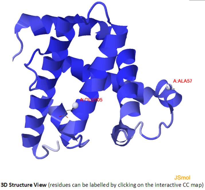
Selecting a point (e.g., A:GLU105, A:ALA57) in the interactive CC map will label the Cα atoms (shown as spheres and same color as selected point) of the pair of residues in the 3D J(s)mol window.
2.6. Collectivity of slow modes
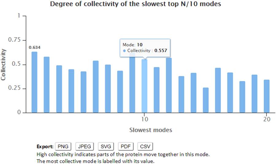
The degree of collectivity of a given mode measures the extent to which the structural elements move together in that particular mode. A high degree of collectivity means a highly cooperative mode, that engages a large portion of (if not the entire) structure. Conversely, low collectivity refers to modes that affect small/local regions only. Modes of high degree of collectivity are generally of interest as functionally relevant modes. These are usually found at the low frequency end of the mode spectrum. The degree of collectivity of these low frequency modes is given by a bar plot, shown below. Hovering over the bar of each mode will display the mode number and its corresponding degree of collectivity. Users may select and enlarge a range of modes in the bar plot, and the figure and data can be exported in different formats using the export buttons.
The nodes files in PDB format, network topology and GNM Kirchhoff matrix used for the GNM calculation are listed. Also, the GNM outputs including eigenvalues, slow modes, fast modes, slow eigenvectors, fast eigenvectors, slow mode average 1-2, slow mode average 1-3 and fast mode average 1-10 are provided. Besides, the text format of cross-correlations (for structures have nodes less than 1000 only), slow modes collectivity, vibrational entropy, theoretical and experiment B-factors along with the scaling factor and the estimated spring constant are provided in the text format.
Descriptions for the plain text files
|
Filename |
Description |
|
(PDB Code)_nodes.pdb |
The GNM nodes file in PDB format. |
|
(PDB Code)_connectivity.txt |
The connectivity (topology) of model in sparse form. 3 columns, comprising two nodes indices columns and a connectivity type column (1, 2 and 3 refer to the connection between amino acid pairs, nucleotides pairs and amino acid – nucleotide pairs, respectively). |
|
(PDB Code).kdat |
The GNM Kirchhoff matrix in sparse form. |
|
(PDB Code).cont |
It lists the number of neighbors are in contact with a specific residue within a cutoff of 7.3 Å |
|
(PDB Code)_resnum.txt |
It contains the number of nodes in the model. |
|
(PDB Code).bfactor |
This file contains the theoretical and experimental B-factors (temperature factors). It has 5 columns. The columns 1 to 3 refer to chain identifiers, residue names and residue indices, respectively; column 4 and 5 are the GNM calculated theoretical B-factors and the x-ray crystallographic b-factors taken from the PDB file. |
|
(PDB Code)_scaling.txt |
The prefactor to scale theoretical fluctuations to experimental B-factors. |
|
(PDB Code)_gamma.txt |
Estimated value of spring constant. |
|
(PDB Code).eigen |
It lists N eigenvalues in the increasing order. The 1st eigenvalue is a zero value. |
|
(PDB Code)_entropy.txt |
The GNM-defined vibrational entropy based on Karplus’ method (1981). |
|
(PDB Code).slowmodes |
23 or more (to keep 40% of the spectrum) columns. The 1-3 columns refer to chain identifiers, residue names and residue indices, respectively; columns 4-23 (or more) are slow mode shapes associated with the 20 (or more) slowest (lowest frequency) modes, starting from the slowest (first) mode. |
|
(PDB Code).slow2av |
4 columns. The 1-3 columns refer to chain identifiers, residue names and residue indices, respectively; column 4 is the residue mean-square fluctuations driven by the joint contribution of the slowest two modes. |
|
(PDB Code).slow3av |
4 columns. The 1-3 columns refer to chain identifiers, residue names and residue indices, respectively; column 4 is the residue mean-square fluctuations driven by the joint contribution of the slowest three modes. |
|
(PDB Code).slow10av |
4 columns. The 1-3 columns refer to chain identifiers, residue names and residue indices, respectively; column 4 is the residue mean-square fluctuations driven by the joint contribution of the slowest ten modes. |
|
(PDB Code).fastmodes |
23 columns. The 1-3 columns refer to chain identifiers, residue names and residue indices, respectively; columns 4-23 are fast mode shapes associated with the 20 fastest (highest frequency) modes, starting from the highest mode. Since the last modes reflect localized fast motions in the protein, these modes have only a few non-zero elements. |
|
(PDB Code).fast10av |
4 columns. The 1-3 columns refer to chain identifiers, residue names and residue indices, respectively; column 4 lists the residue mean-square fluctuations driven by 10 modes having the highest frequency. |
|
(PDB Code).sloweigenvectors |
23 columns. The 1-3 columns refer to chain identifiers, residue names and residue indices, respectively; columns 4-23 are the elements of eigenvectors associated with the 20 slowest (lowest frequency) modes, starting from the slowest (first) mode (column 4). |
|
(PDB Code).fasteigenvectors |
23 columns. The 1-3 columns refer to chain identifiers, residue names and residue indices, respectively; columns 4-23 are the elements of eigenvectors associated with the 20 fastest (highest frequency) modes, starting from the highest mode (column 4). |
|
(PDB Code)_cc_all.txt |
The file contains the cross-correlations for all modes between residue fluctuations. The values are between +1 (perfect concerted motion) and -1 (perfect anti-correlated motions). The file is provided for structures having no more than 1000 nodes only. |
|
(PDB Code) .collectivity-slow |
The file contains N/10 (N is the nodes number) or at least 20 collectivity values of the slowest modes. |
Karplus,M. and Kushick,J.N. (1981) Method for estimating the configurational entropy of macromolecules. Macromolecules, 14, 325-332.
Zimmermann, M.T., Leelananda, S.P., Kloczkowski, A. and Jernigan, R.L. (2012) Combining Statistical Potentials with Dynamics-Based Entropies Improves Selection from Protein Decoys and Docking Poses. J. Phys. Chem. B, 116, 6725-6731.
Ming, D. and Wall, M.E. (2005) Allostery in a coarse-grained model of protein dynamics. Phys. Rev. Lett., 95, 198103.
Dobbins, S.E., Lesk, V.I. and Sternberg, M.J.E. (2008) Insights into protein flexibility: The relationship between normal modes and conformational change upon protein–protein docking. Proceedings of the National Academy of Sciences, 105, 10390-10395.
Particularly,
the vibrational entropy is calculated as
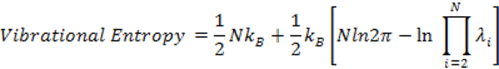
where kB is Boltzmann constant; λi is the eigenvalue of the ith mode; N is the number of nodes of the structure. For example, the GNM-defined vibrational entropy of PDB 101M is -294.07 kB.
Karplus,M. and Kushick,J.N. (1981) Method for estimating the configurational entropy of macromolecules. Macromolecules, 14, 325-332.
The collectivity is defined as
![]()
where, k is the mode number; N is the number of nodes of the structure; ΔRi is the displacement of the ith residue. If Collectivity = 1, the residues have equal contribution in the kth mode; if it is 1/N, it means that only one node contributes to the fluctuation.
Brüschweiler,R. (1995) Collective protein dynamics and nuclear spin relaxation. J. Chem. Phys., 102, 3396-3403.